“所有数值计算归根结底是一系列有限的可微算子的组合”
——《An introduction to automatic differentiation》
符号语言的导数
《Deep Learning》 Chap 6.5.5
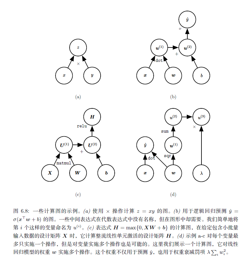
代数表达式和计算图都对符号(symbol) 或不具有特定值的变量进行操作。这些代数或者基于图的表达式被称为符号表示(symbolic representation)。
当我们实际使用或者训练神经网络时,我们必须给这些符号赋值。我们用一个特定的数值(numeric value) 来替代网络的符号输入x,例如 $[1.2, 3, 765, -1.8]^T$。
符号到数值的微分
一些反向传播的方法采用计算图和一组用于图的输入的数值,然后返回在这些输入值处梯度的一组数值。我们将这种方法称为‘‘符号到数值’’ 的微分。这种方法用在诸如Torch(Collobert et al., 2011b)和Caffe(Jia, 2013)之类的库中。
符号到符号的微分
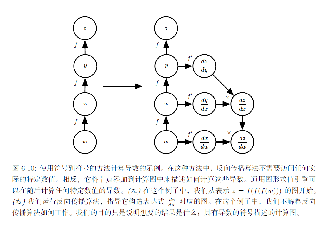
另一种方法是采用计算图以及添加一些额外的节点到计算图中,这些额外的节点提供了我们所需导数的符号描述。这是Theano(Bergstra et al., 2010b; Bastien et al., 2012b) 和TensorFlow(Abadi et al., 2015) 采用的方法。图6.10 中给出了该方法如何工作的一个例子。这种方法的主要优点是导数可以使用与原始表达式相同的语言来描述。
TensorFlow中实现的自动求导(automatic gradient / Automatic Differentiation):
实现的方式是利用反向传递与链式法则建立一张对应原计算图的梯度图。因为导数只是另外一张计算图,可以再次运行反向传播,对导数再进行求导以得到更高阶的导数。(这里我们重点讲这一种,所以下面几个小节会对反向传递算法与链式法则作简要概述)
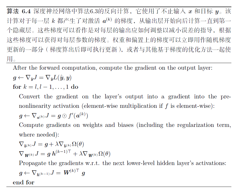
Backpropagation algorithm
【Reference】 http://neuralnetworksanddeeplearning.com/chap2.html
- Input $x$ : Set the corresponding activation $a^1$ for the input layer.
- Feedforward : For each $l=2,3,…,L$ compute $z^l = w^la^{l-1}+b^l$ and $a^l = \sigma (z^l)$
- Output error $\delta^L$ : Compute the vector $\delta^L = \nabla_aC \bigodot \sigma^\prime(z^L)$
- Backpropagate the error : For each $l=L-1,L-2,…,2$ compute $\delta^l = ((w^{l+1})^{\top} \delta^{l+1}) \bigodot \sigma^\prime(z^l)$
- Output : The gradient of the cost function is given by $\frac{\partial C}{\partial w_{jk}^l} = a_k^{l-1}\delta_j^l$ and $\frac{\partial C}{\partial b_{j}^l} = \delta_j^l$
- We’ll use $w_{jk}^l$ to denote the weight for the connection from the kthkth neuron in the $(l-1)^{th}$ layer to the $j^{th}$ neuron in the $l^{th}$ layer.
- We use $b_j^l$ for the bias of the $j^{th}$ neuron in the $l^{th}$ layer. And we use $a_j^l$ for the activation of the $j^{th}$ neuron in the $l^{th}$ layer.
- We use $s \bigodot t$ to denote the elementwise product of the two vectors. Thus the components of $s \bigodot t$ are just $(s \bigodot t)_j=s_j t_j$
Automatic Differentiation
CSE599G1: Deep Learning System (陈天奇)
微分求解大致可以分为4种方式:
手动求解法(Manual Differentiation)
- 求解出梯度公式,然后编写代码,代入实际数值,得出真实的梯度。在这样的方式下,每一次我们修改算法模型,都要修改对应的梯度求解算法,因此没有很好的办法解脱用户手动编写梯度求解的代码。
数值微分法(Numerical Differentiation)
- 不能完全消除truncation error,只是将误差减小。但是由于它实在是太简单实现了,于是很多时候,我们利用它来检验其他算法的正确性,比如在实现backprop的时候,我们用的”gradient check”就是利用数值微分法。
符号微分法(Symbolic Differentiation)
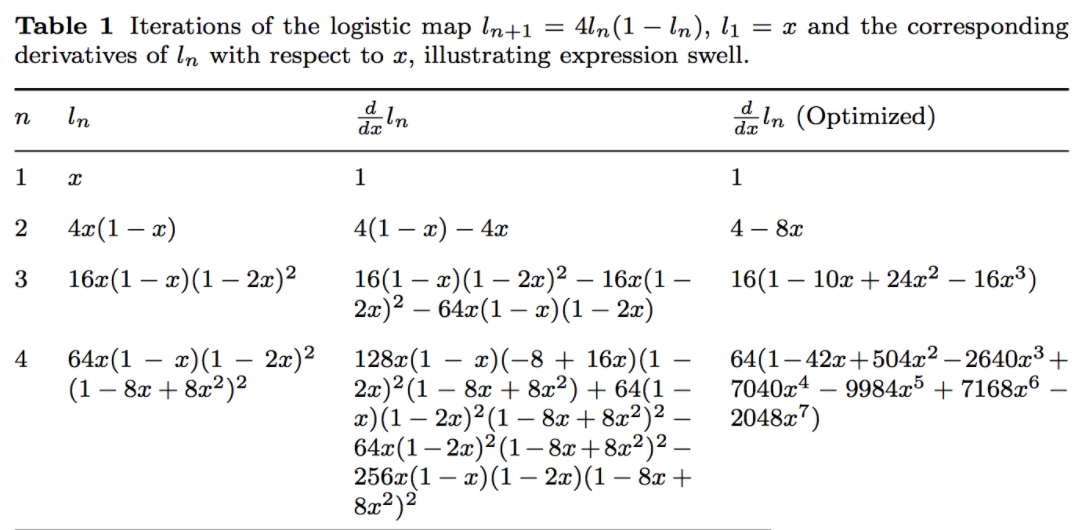
- “表达式膨胀”(expression swell)问题,如果不加小心就会使得问题符号微分求解的表达式急速“膨胀”,导致最终求解速度变慢,如本小节末的图表
Table 1所示。 - Implement differentiation rules:
- Product Rule: $\frac{d(f+g)}{dx}=\frac{df}{dx}+\frac{dg}{dx}$
- Sum Rule: $\frac{d(fg)}{dx}=\frac{df}{dx}g+f\frac{dg}{dx}$
- Chain Rule: $\frac{d(h(x))}{dx}=\frac{df(g(x))}{dx}+\frac{dg(x)}{x}$
- “表达式膨胀”(expression swell)问题,如果不加小心就会使得问题符号微分求解的表达式急速“膨胀”,导致最终求解速度变慢,如本小节末的图表
自动微分法(Automatic Differentiation)
- 自动微分法是一种介于符号微分和数值微分的方法:数值微分强调一开始直接代入数值近似求解;符号微分强调直接对代数进行求解,最后才代入问题数值;自动微分将符号微分法应用于最基本的算子,比如常数,幂函数,指数函数,对数函数,三角函数等,然后代入数值,保留中间结果,最后再应用于整个函数。因此它应用相当灵活,可以做到完全向用户隐藏微分求解过程,由于它只对基本函数或常数运用符号微分法则,所以它可以灵活结合编程语言的循环结构,条件结构等,使用自动微分和不使用自动微分对代码总体改动非常小,并且由于它的计算实际是一种图计算,可以对其做很多优化,这也是为什么该方法在现代深度学习系统中得以广泛应用。
Backpropagation vs AutoDiff (reverse)
CSE599G1 DeepLearning System Lecture4 —— [Slides View](/assets/CSE599G1 DeepLearning System Lecture4.pdf)
- We can take derivative of derivative nodes in autodiff, while it’s much harder to do so in backprop.
- In autodiff, there’s only a forward pass (vs. forward-backward in backprop). So it’s easier to apply graph and schedule optimization to a single graph.
- In backprop, all intermediate results might be used in the future, so we need to keep these values in the memory. On the other hand, in autodiff, we already know the dependencies of the backward graph, so we can have better memory optimization.
Jacobi与链式法则
《Deep Learning》 Chap 6.5.2
该段引用了较多开源社区中对 Deep Learning 一书的中文翻译
https://github.com/exacity/deeplearningbook-chinese
微积分中的链式法则(为了不与概率中的链式法则相混淆)用于计算复合函数的导数。反向传播是一种计算链式法则的算法,使用高效的特定运算顺序。
设 $x$ 是实数, $f$ 和 $g$ 是从实数映射到实数的函数。假设 $y = g(x)$ 并且 $z =f(g(x)) = f(y)$ 。那么链式法则是说
$$\frac{dz}{dx}=\frac{dz}{dy} \frac{dy}{dx}$$
我们可以将这种标量情况进行扩展。 假设$ x\in \mathbb{R}^m, y\in \mathbb{R}^n$,$g$是从$\mathbb{R}^m$到$\mathbb{R}^n$的映射,$f$是从$\mathbb{R}^n$到$\mathbb{R}$的映射。 如果$ y=g(x)$并且$z=f(y)$,那么
$$\frac{\partial z}{\partial x_i} = \sum_j \frac{\partial z}{\partial y_j} \frac{\partial y_j}{\partial x_i}.$$
使用向量记法,可以等价地写成
$$\nabla_{x}z = \left ( \frac{\partial y}{\partial x} \right )^\top \nabla_{y} z,$$
通常我们不将反向传播算法仅用于向量,而是应用于任意维度的张量。从概念上讲,这与使用向量的反向传播完全相同。唯一的区别是如何将数字排列成网格以形成张量。
我们可以想象,在我们运行反向传播之前,将每个张量变平为一个向量,计算一个向量值梯度,然后将该梯度重新构造成一个张量。从这种重新排列的观点上看,反向传播仍然只是将 $Jacobi$ 矩阵乘以梯度。
如果 $Y=g(X)$ 并且 $z=f(Y)$,那么
$$\nabla_X z = \sum_j (\nabla_X Y_j)\frac{\partial z}{\partial Y_j}. $$
于是,反向传播算法就变得非常简单:
为了计算某个标量 $z$ 关于图中它的一个祖先 $x$ 的梯度,我们首先观察到它关于 $z$ 的梯度由 $\frac{dz}{dz}=1$ 给出。 然后,我们可以计算对图中 $z$ 的每个父节点的梯度,通过现有的梯度乘以产生$z$的操作的 $Jacobian$。 我们继续乘以 $Jacobian$,以这种方式向后穿过图,直到我们到达 $x$。 对于从 $z$ 出发可以经过两个或更多路径向后行进而到达的任意节点,我们简单地对该节点来自不同路径上的梯度进行求和。
Tensorflow的自动求导实现
Tensorflow 中的符号求导见项目下的 tensorflow/python/ops/gradients_impl.py
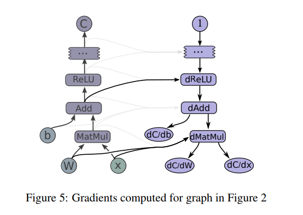
“Constructs symbolic derivatives of sum ofysw.r.t. x inxs”[db, dW, dx] = tf.gradients(C, [b,W,x])
《Deep Learning》一书中,表示Theano与Tensorflow采用如下图算法的子程序来建立 $grad_table$,而在Tensorflow白皮书的第五节中,介绍了在$grad_table$中,存储了通常会被重复计算多次的 $ \partial u^{(n)} / \partial u^{(i)}$,用以减少程序的冗余计算从而增加效率:
If a tensor $C$ in a TensorFlow graph depends, perhaps through a complex subgraph of operations, on some set of tensors $X_k$, then there is a built-in function that will return the tensors ${dC/dX_k}$.
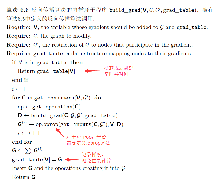
每个操作 $op$ 也与 $bprop$ 操作相关联。该 $bprop$ 操作可以计算如上述公式所描述的 $Jacobi$ 向量积。这是反向传播算法能够实现很大通用性的原因。每个操作负责了解如何通过它参与的图中的边来反向传播。反向传播算法本身并不需要知道任何微分法则。它只需要使用正确的参数调用每个操作的 $bprop$ 方法即可。正式地,$op.bprop(inputs,X,G)$ 必须返回
$$ \sum_i (\nabla_{X} \verb|op.f(inputs|)_i) \textsf{G}_i, $$
这里,$inputs$ 是提供给操作的一组输入,$op.f$ 是操作实现的数学函数,$X$ 是输入,我们想要计算关于它的梯度,$G$ 是操作对于输出的梯度。
$op.bprop$ 方法应该总是假装它的所有输入彼此不同,即使它们不是。例如,如果 $mul$ 操作传递两个 $x$ 来计算 $x^2$,$op.bprop$ 方法应该仍然返回 $x$ 作为对于两个输入的导数。反向传播算法后面会将这些变量加起来获得 $2x$,这是 $x$ 上总的正确的导数。
反向传播算法的软件实现通常提供操作和其 $bprop$ 两种方法,所以深度学习软件库的用户能够对使用诸如矩阵乘法、指数运算、对数运算等等常用操作构建的图进行反向传播。构建反向传播新实现的软件工程师或者需要向现有库添加自己的操作的高级用户通常必须手动为新操作推导 $op.bprop$ 方法。
我们以 $Tensorflow$ 的一次 commit: * Register log1p in math_ops. 为例:
1 | // 该文件为 tensorflow/core/ops/math_ops.cc |
1 | # 该文件为 tensorflow/python/ops/math_grad.py |
由于重复子表达式的存在,简单的算法可能具有指数运行时间。现在我们已经详细说明了反向传播算法,我们可以去理解它的计算成本:
对于与 $Theano$ 与 $Tensorflow$ 类似的平台,反向传播算法在原始图的每条边添加一个 $Jacobi$ 向量积,可以用 $O(1)$ 个节点来表达。因为计算图是有向无环图,它至多有 $O(n^2)$ 条边。
而对于实践中常用的图的类型,情况会更好:大多数神经网络的代价函数大致是链式结构的,使得反向传播只有 $O(n)$ 的成本。这远远胜过简单的方法,简单方法可能需要执行指数级的节点。这种潜在的指数级代价可以通过非递归地扩展和重写递归链式法则看出:
$$ \frac{\partial u^{(n)}}{\partial u^{(j)}} =
\sum_{\substack{\text{path}(u^{(\pi_1)}, u^{(\pi_2)}, \ldots, u^{(\pi_t)} ),\ \text{from } \pi_1=j \text{ to }\pi_t = n}}
\prod_{k=2}^t \frac{\partial u^{(\pi_k)}}{\partial u^{(\pi_{k-1})}}. $$
由于节点 $j$ 到节点 $n$ 的路径数目可以关于这些路径的长度上指数地增长,所以上述求和符号中的项数(这些路径的数目),可能以前向传播图的深度的指数级增长。 会产生如此大的成本是因为对于 $\frac{\partial u^{(i)}}{\partial u^{(j)}}$ ,相同的计算会重复进行很多次。为了避免这种重新计算,我们可以将反向传播看作一种表填充算法,利用存储的中间结果 $\frac{\partial u^{(n)}}{\partial u^{(i)}}$ 来对表进行填充。 图中的每个节点对应着表中的一个位置,这个位置存储对该节点的梯度。 通过顺序填充这些表的条目,反向传播算法避免了重复计算许多公共子表达式——这种表填充策略有时被称为动态规划。
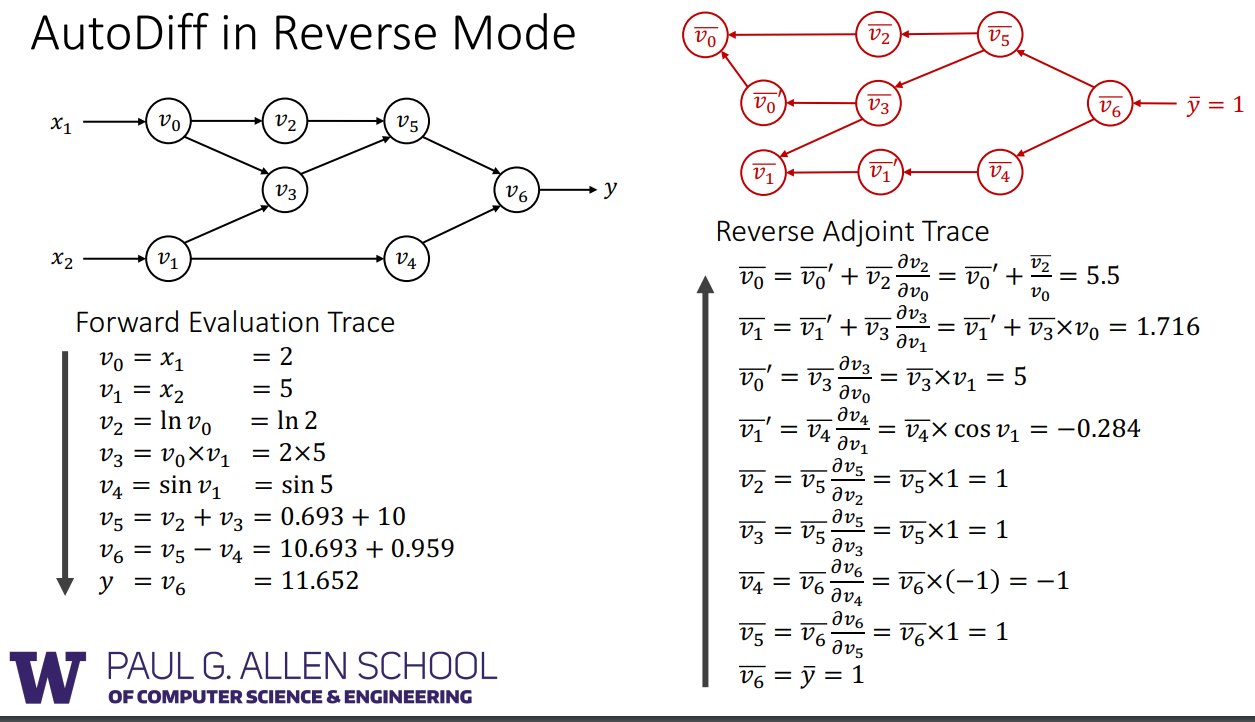
上述AutoDiff的图片来自于:http://dlsys.cs.washington.edu/pdf/lecture4.pdf
高阶导数
一些软件框架支持使用高阶导数。在深度学习软件框架中,这至少包括Theano和TensorFlow。这些库使用一种数据结构来描述要被微分的原始函数,它们使用相同类型的数据结构来描述这个函数的导数表达式。这意味着符号微分机制可以应用于导数(从而产生高阶导数)。
黑塞矩阵(Hessian Matrix),又译作海森矩阵、海瑟矩阵、海塞矩阵等,是一个多元函数的二阶偏导数构成的方阵,描述了函数的局部曲率。黑塞矩阵最早于19世纪由德国数学家Ludwig Otto Hesse提出,并以其名字命名。黑塞矩阵常用于牛顿法解决优化问题,利用黑塞矩阵可判定多元函数的极值问题。 —— 百度百科
在深度学习的相关领域,很少会计算标量函数的单个二阶导数。 相反,我们通常对Hessian矩阵的性质比较感兴趣。 如果我们有函数 $f:\mathbb{R}^n \to \mathbb{R}$,那么Hessian矩阵的大小是 $n\times n$。 在典型的深度学习应用中,$n$ 将是模型的参数数量,可能很容易达到数十亿。 因此,完整的Hessian矩阵甚至不能表示。
典型的深度学习方法是使用Krylov方法,而不是显式地计算Hessian矩阵。 Krylov方法是用于执行各种操作的一组迭代技术,这些操作包括像近似求解矩阵的逆、或者近似矩阵的特征值或特征向量等,而不使用矩阵-向量乘法以外的任何操作。
为了在Hesssian矩阵上使用Krylov方法,我们只需要能够计算Hessian矩阵 $H$ 和一个任意向量 $v$ 间的乘积即可(该表达式中两个梯度的计算都可以由适当的软件库自动完成):
$$ H v=\nabla_{x} \left [ (\nabla_{x} f(x))^\top v\right ] $$
虽然计算Hessian通常是不可取的,但是可以使用Hessian向量积。 可以对所有的 $i=1,\ldots,n$ 简单地计算 $H e^{(i)}$,其中 $e^{(i)}$ 是 $e_i^{(i)}=1$ 并且其他元素都为 $0$ 的 one-hot 向量(通过阅读源码,我们发现Hessian向量积 $Hv$ 尚未实现成avaliable的状态,Tensorflow当前版本当前仅对Hesssian矩阵完成了实现)。
其它:PyTorch的自动求导
PyTorch提供了包torch.autograd用于自动求导。在前向过程中,PyTorch会构建计算图,每个节点用Variable表示,边表示由输入节点到输出节点的函数(torch.autograd.Function对象)。Function对象不仅负责执行前向计算,在反向过程中,每个Function对象会调用.backward()函数计算输出对输入的梯度,然后将梯度传递给下一个Function对象。
How autograd encodes the history (PyTorch)
原文 Internally, autograd represents this graph as a graph of
Functionobjects (really expressions), which can beapply()ed to compute the result of evaluating the graph. When computing the forwards pass, autograd simultaneously performs the requested computations and builds up a graph representing the function that computes the gradient (the.grad_fnattribute of eachVariableis an entry point into this graph). When the forwards pass is completed, we evaluate this graph in the backwards pass to compute the gradients.
An important thing to note is that the graph is recreated from scratch at every iteration, and this is exactly what allows for using arbitrary Python control flow statements, that can change the overall shape and size of the graph at every iteration. You don’t have to encode all possible paths before you launch the training - what you run is what you differentiate.
http://pytorch.org/docs/master/notes/autograd.html#how-autograd-encodes-the-history
自动求导如何编码历史信息 in PyTorch-CN
每个变量都有一个.creator属性,它指向把它作为输出的函数。这是一个由Function对象作为节点组成的有向无环图(DAG)的入口点,它们之间的引用就是图的边。每次执行一个操作时,一个表示它的新Function就被实例化,它的forward()方法被调用,并且它输出的Variable的创建者被设置为这个Function。然后,通过跟踪从任何变量到叶节点的路径,可以重建创建数据的操作序列,并自动计算梯度。
需要注意的一点是,整个图在每次迭代时都是从头开始重新创建的,这就允许使用任意的Python控制流语句,这样可以在每次迭代时改变图的整体形状和大小。在启动训练之前不必对所有可能的路径进行编码—— what you run is what you differentiate.
PyTorch中定义一个新操作
定义新的操作,意味着定义Function的子类,并且这些子类必须重写以下函数:::forward()和::backward()。初始化函数::__init__()根据实际需求判断是否需要重写。
forward()
forward()可以有任意多个输入、任意多个输出,但是输入和输出必须是Variable。backward()
backward()的输入和输出的个数就是forward()函数的输出和输入的个数。其中,backward()输入表示关于forward()输出的梯度,backward()的输出表示关于forward()的输入的梯度。在输入不需要梯度时(通过查看needs_input_grad参数)或者不可导时,可以返回None。Reference: http://blog.csdn.net/victoriaw/article/details/72566249
1 | # Inherit from Function |